Mapping embeddings: from meaning to vectors and back

"What I cannot create, I do not understand" ―Richard Feynman

"If you can't explain it simply, you don't understand it well enough." ―Albert Einstein

I'd like to tell you a story involving not one but two very simple visualization tools for exploring document chunks and queries in embedding space: RAGmap 🗺️🔍 and RAGxplorer 🦙🦺.

Don't worry if you didn't get that last paragraph. Understanding the motivation and building enough of an intuition to justify the existence of these tools is why I'm writing this post anyway.

Inspired by DeepLearning.ai's short course on advanced retrieval for AI with Chroma, both tools take a similar approach and use a similar stack, but they differ in some very important ways.

In this post, we'll focus on the threads they have in common and I'll try to make a case for the importance of creating your own tools from scratch, if only to build your own mental models for concepts like embeddings, dimensionality reduction techniques and advanced retrieval mechanisms.

Ready, set... go! 🏃

Introduction to Embeddings

Let's start with the basic question: what are embeddings?

There are some great articles out there on what embeddings are and why they matter. Here's a small sample of pseudo-random definitions I've collected just for this post:

"Embeddings are numerical representations of real-world objects that machine learning (ML) and artificial intelligence (AI) systems use to understand complex knowledge domains like humans do." (AWS)

"Embeddings are vectorial representations of text that capture the semantic meaning of paragraphs through their position in a high dimensional vector space." (Mistral AI)

"Embeddings are vectors that represent real-world objects, like words, images, or videos, in a form that machine learning models can easily process." (Cloudflare)

"learnt vector representations of pieces of data" (Sebastian Bruch)

In a nutshell, embeddings are just an efficient way to encode data in numerical form. These encodings are tied to a specific embedding model that turns raw data like text, images, or video, into a vector representation.

RAGmap has built-in support for embedding models from Amazon Bedrock ⛰️ and Hugging Face 🤗, while RAGxplorer uses OpenAI:

1
2
3
4
5
6
7
8
9
10
11
12
13
14
15
16
"""
Retrieves information about the embedding models
available in Amazon Bedrock
"""

import json
import boto3

bedrock = boto3.client("bedrock")

response = bedrock.list_foundation_models(
    byOutputModality="EMBEDDING",
    byInferenceType="ON_DEMAND"
)

print(json.dumps(response['modelSummaries'], indent=4))

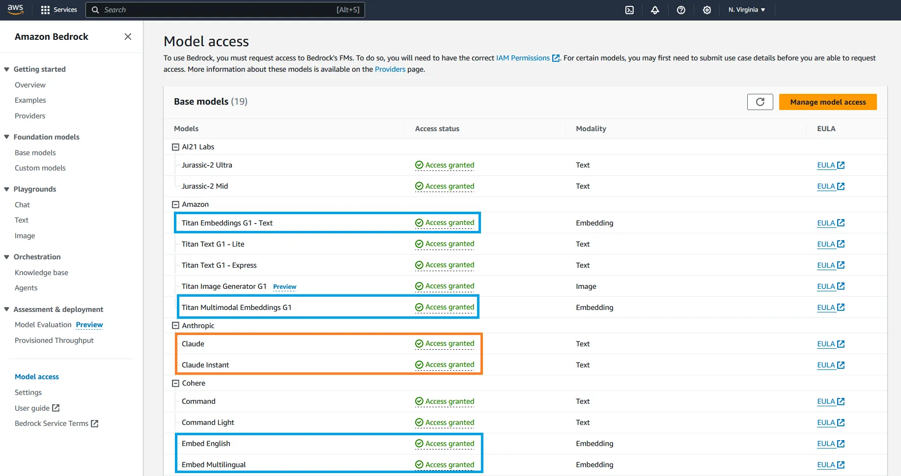
As of this writing, Amazon Bedrock offers access to embedding models from Cohere and Amazon Titan:

🧐 Interested in training your own embedding model? Check out this article from Hugging Face on how to Train and Fine-Tune Sentence Transformers Models.

1
2
3
4
5
6
7
8
9
10
11
12
13
14
15
16
17
18
19
20
21
22
23
24
25
26
27
28
29
30
31
32
33
34
35
36
37
38
39
40
41
42
43
44
45
46
47
48
49
50
51
52
53
54
55
56
57
58
59
60
61
62
63
64
65
66
67
68
69
70
71
72
73
74
75
76
77
78
79
80
81
82
83
84
85
86
87
88
89
90
91
92
93
94
95
96
97
98
99
100
101
[
    {
        "modelArn": "arn:aws:bedrock:us-east-1::foundation-model/amazon.titan-embed-g1-text-02",
        "modelId": "amazon.titan-embed-g1-text-02",
        "modelName": "Titan Text Embeddings v2",
        "providerName": "Amazon",
        "inputModalities": [
            "TEXT"
        ],
        "outputModalities": [
            "EMBEDDING"
        ],
        "customizationsSupported": [],
        "inferenceTypesSupported": [
            "ON_DEMAND"
        ],
        "modelLifecycle": {
            "status": "ACTIVE"
        }
    },
    {
        "modelArn": "arn:aws:bedrock:us-east-1::foundation-model/amazon.titan-embed-text-v1",
        "modelId": "amazon.titan-embed-text-v1",
        "modelName": "Titan Embeddings G1 - Text",
        "providerName": "Amazon",
        "inputModalities": [
            "TEXT"
        ],
        "outputModalities": [
            "EMBEDDING"
        ],
        "responseStreamingSupported": false,
        "customizationsSupported": [],
        "inferenceTypesSupported": [
            "ON_DEMAND"
        ],
        "modelLifecycle": {
            "status": "ACTIVE"
        }
    },
    {
        "modelArn": "arn:aws:bedrock:us-east-1::foundation-model/amazon.titan-embed-image-v1",
        "modelId": "amazon.titan-embed-image-v1",
        "modelName": "Titan Multimodal Embeddings G1",
        "providerName": "Amazon",
        "inputModalities": [
            "TEXT",
            "IMAGE"
        ],
        "outputModalities": [
            "EMBEDDING"
        ],
        "customizationsSupported": [],
        "inferenceTypesSupported": [
            "ON_DEMAND"
        ],
        "modelLifecycle": {
            "status": "ACTIVE"
        }
    },
    {
        "modelArn": "arn:aws:bedrock:us-east-1::foundation-model/cohere.embed-english-v3",
        "modelId": "cohere.embed-english-v3",
        "modelName": "Embed English",
        "providerName": "Cohere",
        "inputModalities": [
            "TEXT"
        ],
        "outputModalities": [
            "EMBEDDING"
        ],
        "responseStreamingSupported": false,
        "customizationsSupported": [],
        "inferenceTypesSupported": [
            "ON_DEMAND"
        ],
        "modelLifecycle": {
            "status": "ACTIVE"
        }
    },
    {
        "modelArn": "arn:aws:bedrock:us-east-1::foundation-model/cohere.embed-multilingual-v3",
        "modelId": "cohere.embed-multilingual-v3",
        "modelName": "Embed Multilingual",
        "providerName": "Cohere",
        "inputModalities": [
            "TEXT"
        ],
        "outputModalities": [
            "EMBEDDING"
        ],
        "responseStreamingSupported": false,
        "customizationsSupported": [],
        "inferenceTypesSupported": [
            "ON_DEMAND"
        ],
        "modelLifecycle": {
            "status": "ACTIVE"
        }
    }
]

🤔 Did you know? Long before embeddings became a household name, data was often encoded as hand-crafted feature vectors. These too were meant to represent real-world objects and concepts.

If this all sounds a bit scary, just think of embedding as a bunch of numbers (vectors).

Don't believe me? Let's look at an example...

Last time I was in Madrid, I gave an internal talk about RAGmap and I was thinking about a cool way to demonstrate embedding models to a largely non-technical audience. It was Valentine's day and I was feeling homesick, so I came up with this idea to send a single word to Amazon Titan for Embeddings.

That word was love.

1
2
3
4
5
6
7
8
9
10
11
12
13
14
15
"""
Sends love to Amazon Titan for Embeddings ❤️
and gets numbers in return 🔢
"""

import json
import boto3

bedrock_runtime = boto3.client("bedrock-runtime")
response = bedrock_runtime.invoke_model(
    modelId="amazon.titan-embed-text-v1",
    body="{\"inputText\": \"love\"}"
)
body = json.loads(response.get('body').read())
print(body['embedding'])

love is a great choice for two reasons:

First, most models will represent love with a single token. In the case of Amazon Titan for Embeddings, you can check that this is the case by printing the inputTextTokenCount attribute of the model output (in English, 1 token ~=``4``chars). So what we get is a pure, unadulterated representation of the word.
Second, love is one of the most complex and layered words there is. One has to wonder, looking at the giant vector below, where exactly are we hiding those layers and how can we peel that lovely onion. Where is the actual love?

"Love loves to love love." ―James Joyce

The answer, of course, much like the word itself, lies in connection. The nice thing about these representations, especially when dealing with text (words, sentences, whole documents), is that they preserve (semantic) meaning in a very precise way. This becomes evident when we start playing around and comparing vectors with each other, measuring their "relatedness" to one another.

🔮 The usual way to judge how similar two vectors are is to call a distance function. We won't have to worry about this though, since the vector database we're going to use has built-in support for common metrics viz. Squared Euclidean (L2 Squared) l2, Inner Product ip and Cosine similarity cosine distance functions. If you'd like to change this value (hnsw:space defaults to l2), please refer to Chroma > Usage Guide > Using collections > Changing the distance function.

Now, what if we want to go beyond single words? What if, say, we want to encode all Wikipedia

or turn 100M songs in Amazon Music into vectors so we can search and find similar tracks?

Where would we start?

It is clear that we'll need an efficient way to store all these numbers and search through them. Cue vector databases...

Working with Vector Databases

"The most important piece of the preprocessing pipeline, from a systems standpoint, is the vector database." ―Andreessen Horowitz

"Every database will become a vector database, sooner or later." ―John Hwang

Vector databases seem to be everywhere these days and there is a common misconception going around that it takes a special kind of database just to work with embeddings.

The truth is that any database can be a vector database, so long as it treats vectors as first class citizens.

I strongly believe that every database will eventually become a vector database. This will happen gradually up to a point where the name itself becomes a relic of the past.

At AWS, we've been adding vector storage and search capabilities to our stack of database services, so that customers don't have to migrate or use a separate database just for handling embeddings:

Both RAGmap and RAGxplorer use Chroma, an AI-native open source embedding database, that is very flexible and easy to use. Since we're going to work mostly with small (<10MB) documents chunked into bits of fixed size, this will do just fine.

1
2
3
4
5
6
7
8
9
10
11
12
13
14
15
16
17
18
19
20
21
22
23
24
25
26
27
28
29
30
31
32
33
34
35
36
37
"""
Creates a Chroma collection and indexes some sample sentences
using Amazon Bedrock.

☝️⚠️ As of this writing, Chroma only supports Titan models:
https://github.com/chroma-core/chroma/pull/1675

If you want to use Cohere Embed models, install Chroma by running the command:
> pip install git+https://github.com/JGalego/chroma@bedrock-cohere-embed
"""

import boto3
import chromadb

from chromadb.utils.embedding_functions import AmazonBedrockEmbeddingFunction

# Create embedding function
session = boto3.Session()
bedrock_ef = AmazonBedrockEmbeddingFunction(
	session=session,
	model_name="cohere.embed-multilingual-v3"
)

# Create collection
client = chromadb.Client()
collection = client.create_collection(
	"demo",
	embedding_function=bedrock_ef
)

# Index data samples
collection.add(
	documents=["Hello World", "Olá Mundo"],
	metadatas=[{'language': "en"}, {'language': "pt"}],
	ids=["hello_world", "ola_mundo"]
)
print(collection.peek())

Dimensionality Reduction Techniques

Now, remember those 1536 numbers that we got for love?

Seeing that our puny human brains can't make heads or tails of high-dimensional data, we'll have to turn them into something more manageable.

Fortunately, bringing high-dimensional data to the lower-dimensional realm is something we've been doing for a while now in ML under the moniker of dimensionality reduction.

Source: Adapted from Kobak & Linderman (2021)

There's a veritable smorgasbord of dimensionality reduction techniques which usually fall into one or more of these categories:

global vs local - local methods preserve the local characteristics of the data, while global methods provide an "holistic" view of the data
linear vs non-linear - in general, nonlinear methods can handle very nuanced data and are usually more powerful, while linear methods are more robust to noise.
parametric vs non-parametric - parametric techniques generate a mapping function that can be used to transform new data, while non-parametric methods are entirely "data-driven", meaning that new (test) data cannot be directly transformed with the mapping learnt on the training data.
deterministic vs stochastic - given the same data, deterministic methods will produce the same mapping, while the output of a stochastic method will vary depending on the way you seed it.

There's no perfect dimensionality reduction technique, just like there's no ideal map projection.

Source: adapted from GIS&T Body of Knowledge

They all have their own strengths and weaknesses (check out the poles in the Mercator projection) and they'll work better or worse depending on the data you feed in.

As of this writing, RAGmap supports 3 different dimensionality reduction algorithms:

PCA (Principal Component Analysis) is great for capturing global patterns
t-SNE (t-Distributed Stochastic Neighbor Embedding) emphasizes local patterns and clusters
UMAP (Uniform Manifold Approximation and Projection) can handle complex relationships

The acronyms themselves are not important. What is important is to gain an intuition of their differences. As an example, let's take the woolly mammoth in the room... 🦣

"With four parameters I can fit an elephant, and with five I can make him wiggle his trunk" ―John von Neumann

Looking at the flattened versions of our pachyderm friend, it is clear that UMAP strikes a better balance between local and global structures (just look at those yellow tusks). Nevertheless, both methods introduce a bit of warping of the original data, which means that the projection components aren't directly interpretable as in the case of PCA.

RAG in a nutshell

Finally, I'd like to spend a couple of minutes on the topic of Retrieval Augmented Generation (RAG) seeing that both tools have that in common, starting with the name.

But first, let's recap our journey so far:

Embeddings represent raw data as vectors in a way that preserves meaning
Vector databases can be used to store, search and do all kinds of operations on them
Dimensionality reduction is a good but imperfect way to make them more tangible

Now that we have this incredible "tool" in our arsenal, how can we put it to good use... and when.

As you probably know by now, large language models (LLMs) are trained on HUGE amounts of data, usually measured in the Trillions of tokens. For good or bad, if something exists on the web, there's a good chance these models have already "seen" it.

But, if there's one thing these models haven't seen for sure (hopefully!), it's your own private data. They have no means of accessing your data unless you put it (quite literally) in context.

That's when RAG comes in...

There's so much hype around RAG that a lot of people have a hard time seeing it for what it actually is: a hack, a clever way to connect LLMs and external data.

The general idea goes something like this:

Get your data from where it lives (datalake, database, API, &c.)
Chunk it into smaller pieces that can be consumed by the embeddings model
Send it to an embeddings model to generate the vector representations (indexes)
Store those indexes as well as some metadata in a vector database
(Repeat steps 1-4 for as long as there is new data to index)

User queries received by the LLM are first sent to the embeddings model and then searched within the vector database. Any relevant results are shared with the LLM, along with the original query, so the model can generate a response backed by actual data and send it to the user.

As you'll see in the demo section, RAGmap and RAGxplorer work just like any other RAG-based system with two major differences:

They both work on the scale of a single document, and
There's no LLM involved, just embeddings and their projections.

This makes RAGmap and RAGxplorer great visualization tools for debugging RAG-based applications, if all we care about is identifying "distractors" among the indexed results that will be sent back to the LLM.

👆 There's one notable exception related to advanced retrieval techniques. A naive query search won't always work and we'll need to move on to more advanced methods. As of this writing, RAGmap has built-in support for simple query transformations like generated answers (HyDE) / query --> LLM --> hypothetical answer and multiple sub-queries / query --> LLM --> sub-queries using Anthropic Claude models via Amazon Bedrock.

Demo: RAGmap 🗺️🔍

In this section, I'm going to show you a quick demo involving RAGmap and comment briefly on its implementation.

If you don't want to follow these steps, feel free to watch the video instead 📺

Prerequisites

Before we get started, take some time perform the following prerequisite actions:

Enable access to the embedding (Titan Embeddings, Cohere Embed) and text (Anthropic Claude) models via Amazon Bedrock.

For more information on how to request model access, please refer to the Amazon Bedrock User Guide (Set up > Model access)

Step 0: Start

Let's start by cloning the RAGmap repository, installing the dependencies and running the app:

1
2
3
4
5
6
7
8
9
# Clone the repository
git clone https://github.com/JGalego/RAGmap

# Install dependencies
cd RAGmap
pip install -r requirements.txt

# Start the application
streamlit run app.py

Step 1: Load

The first step is to load a document. I'm going to upload a document containing all Amazon shareholder letters from 1997 to 2017 ✉️, but you're free to chose a different one. RAGmap supports multiple file formats, including PDF, DOCX and PPTX.

Small files 🤏 will be faster to process, but the visualization will not be as memorable. Just don't choose a big file!

Step 2: Index + Store

In the Build a vector database section, you can choose how to break the document apart (chunking strategy), which embedding model to use and how RAGmap is going to project the embeddings into 2D/3D plots (dimensionality reduction).

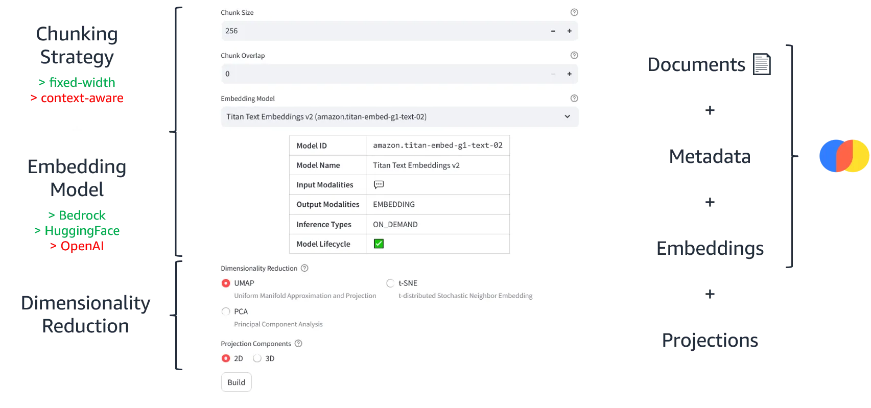
When you're ready, just click Build. Be sure to try different configurations if you have time. Depending on the document size, this should take around 1-2 minutes ⏳.

Step 3: Query

Once the vector database is populated, RAGmap will immediately display a visualization of your document chunks. Let's postpone the end result for a moment to check the Query section.

Just as a reminder, RAGmap supports both naive search and query transformations as retrieval strategies. If you're using any of the advanced techniques, make sure you have enough permissions to call Claude models via Amazon Bedrock.

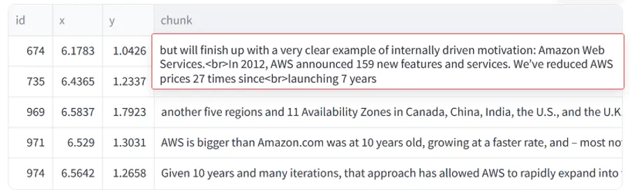
Just type in a query e.g. How many services and features were released by AWS in 2012?, select a retrieval method and hit Search.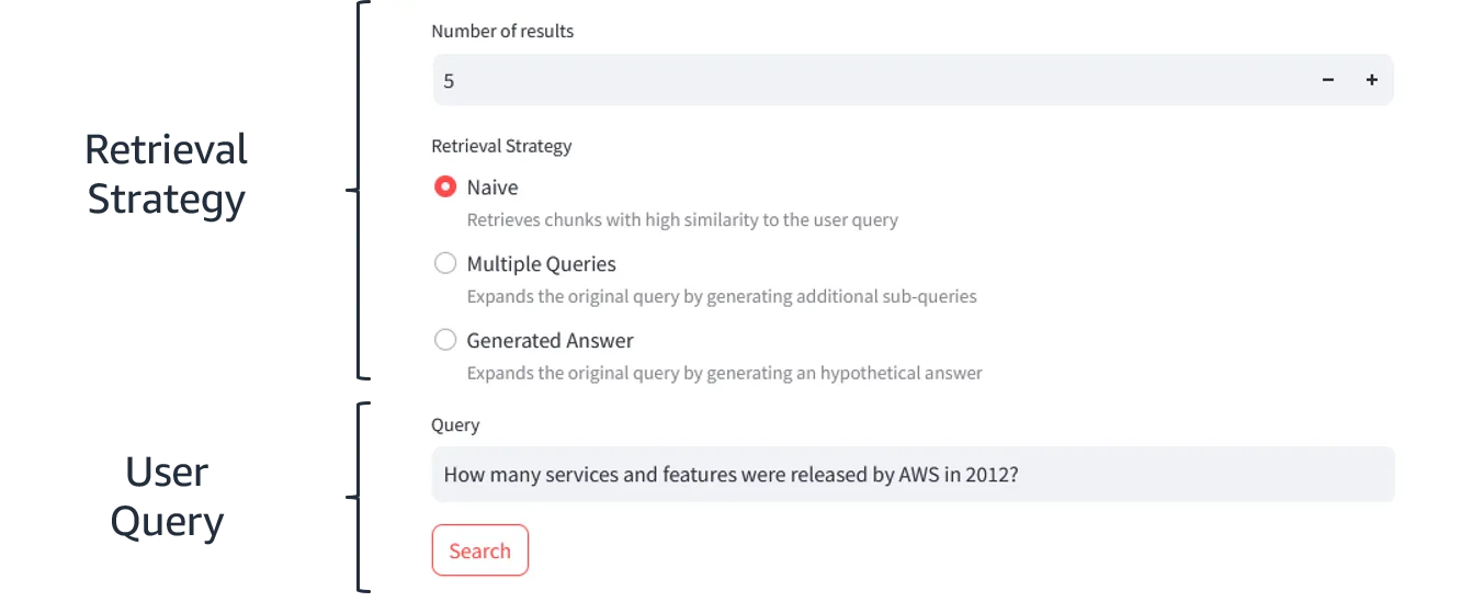

Step 4: Evaluate

Looking at the image below, our query is close to the retrieved results, which is what we would expect.

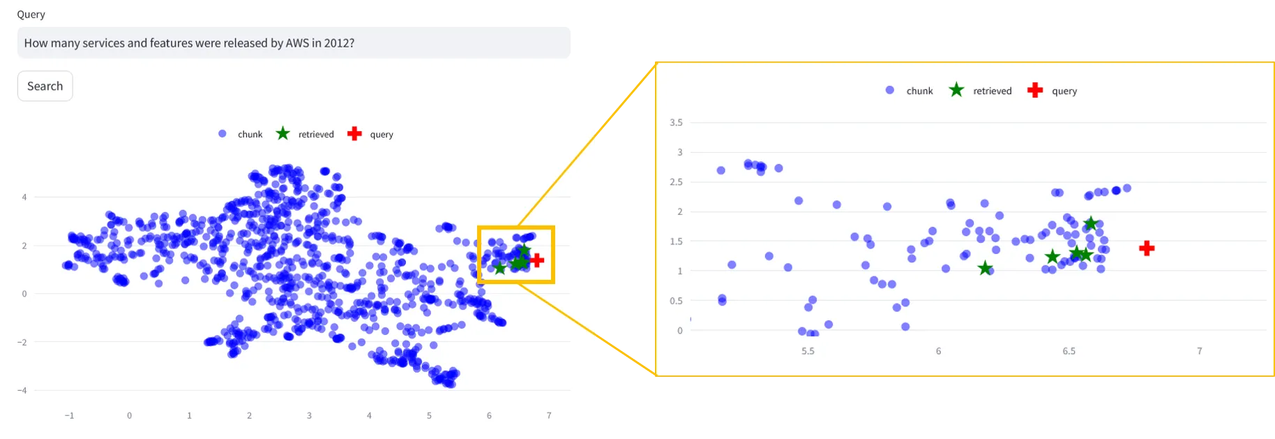
Notice, however, that the retrieved indexes are not the ones closest to our query. Since we're using distance measures, that operate on the whole embeddings, to find relevant results, but plotting warped (projected) versions of those embeddings, this is also reasonable. Both UMAP and t-SNE will try to preserve local distances, so we don't expect them to be too far off, say on opposite sides of the plot.

Fun fact: the first critical bug 🐛 in RAGxplorer was caught thanks to RAGmap. While testing both tools, I noticed that the retrieved IDs were too far away from the original query and were inconsistent with the results I was getting from RAGmap. Since the tools use different models - RAGmap (Amazon Bedrock, Hugging Face) and RAGxplorer (OpenAI) - there was bound to be a difference, but not one this big. It turns out that the issue was related to the way chroma returns documents and orders them.

Finally, as an additional check, we can validate that the returned chunks are relevant to our original query.

Thanks for sticking around, see you next time! 👋

References 📚

Code 👨‍💻

Courses 👩‍🏫

Miscellaneous 👾

(Arize) Embeddings: meaning, examples and how to compute
(Mistral) Embeddings
(Cloudflare) What are embeddings in machine learning?
(Hugging Face) Train and fine-tune sentence transformer models
(Cohere) The Embedding archives: millions of wikipedia article embeddings in many languages
(a16z) Emerging architectures for LLM applications
(PAIR) Understanding UMAP
(Latent Space) RAG is a Hack
(TruLens) The RAG Triad
<shameless-plug>A Tour of GenAI</shameless-plug>

Any opinions in this post are those of the individual author and may not reflect the opinions of AWS.

Site Terms, Privacy, and more.